MATLAB Deep Learning | Part Two | Transfer Learning1. Transfer Learning
The purpose of a transfer learning is to fine-tune a pre-trained Convolutional Neural Network that will be used to perform classification on a new problem. According Mathworks, "AlexNet has been trained on over a million images and can classify images into 1000 object categories (such as keyboard, coffee mug, pencil, and many animals)." However, if we are looking for a classification accuracy over 99% on given objects, we have to perform transfer learning. Transfer learning is commonly used in deep learning applications that we can take a pretrained network and use it as a starting point to learn new tasks. Fine-tuning a network with transfer learning is usually much faster and easier than training a network with randomly initialized weights from scratch. We can quickly transfer the learned features onto a new task using a smaller number of training images (aka ImageDataStore). 2. Deep learning | Project # 2 | Transfer Learning
In this project, we will create a new Data Store of images with five labels that are related to our problem, re-train the selected CNN with the new images (also called transfer learning), and we will perform object classification using the new CNN. 2a) Select the appropriate base CNN Select a CNN that is close to your problem statement to re-train it or perform a transfer learning on the selected CNN. Additionally, MathWorks has provided the following chart to compare the validation accuracy of different CNNs along with the GPU time required to make a prediction. 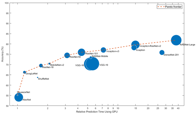
Prediction Accuracy and GPU time: This chart shows Classification accuracy and GPU prediction time of different CNNs.
While choosing a CNN, there will be a trade-off between network accuracy, speed, and size. Another limitation while trying to perform a transfer learning is the prediction time using on a CPU. If you try to use a CPU, the prediction time is extremely high. However, using a Graphics Processing Unit (GPU) instead of CPU will make the transfer learning much faster. Considering all the above parameters, select the approprate CNN for your model.
In our case, we have selected GoogLeNet. Note: if your computer doesn't have a GPU, working with a CPU for transfer learning is time consuming and tedious. 2b) Creating Image DataStore
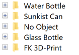
Using the Matlab script shown below, you can create a Data store of 1000 images for each object (aka labels) and store the images into their designated file folders. In this example, pictures are taken at an interval of one second and the pictures will be stored inside designitaed sub-folders under the main folder.
%% Automatic Picture taker After creating the DataStore of images, use the following code blocks to perform a successive transfer learning and validation test on your classification objects.
2c) Transfer Learning Using GoogLeNet
Download the function "findLayersToReplace" from here findlayerstoreplace.m and save the function inside the project folder you are working on. The function can also be downloaded from MathWorks website.
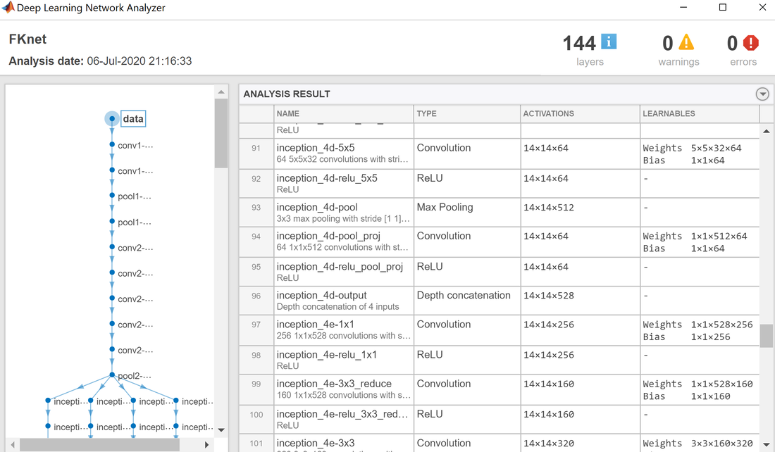
%{ After running the above code, you will get the "Deep Learning Network Analyzer" chart. You can observe from this chart that googLeNet has 144 layers and the transfer learning is performed on the last two fully-connected layers. Close the Analyzer chart and continue performing the transfer learning.
Transfer the layers to the new classification task
numClasses = numel(categories(imdsTrain.Labels)); After running the above code, download the second function, "freezeWeights" from here freezeweights.m and the third function, "createLgraphUsingConnections" from here createlgraphusingconnections.m and make sure to save these functions inside the project folder you are working on.
Train The Network
Start traning the network using the code below. Specify the training options as shown in the code. For transfer learning, keep the features from the early layers of the pretrained network (the transferred layer weights). To slow down learning in the transferred layers, set the initial learning rate to a small value. When performing transfer learning, you do not need to train for as many epochs. An epoch is a full training cycle on the entire training data set. Specify the mini-batch size and validation data. Matlab will validate the network every ValidationFrequency iterations during training. Train the network that consists of the transferred and new layers. By default, trainNetwork uses a GPU if one is available (requires Parallel Computing Toolbox™ and a CUDA® enabled GPU with compute capability 3.0 or higher). Otherwise, it uses a CPU.
%% Start training the new network with the selected options
%% Training Results
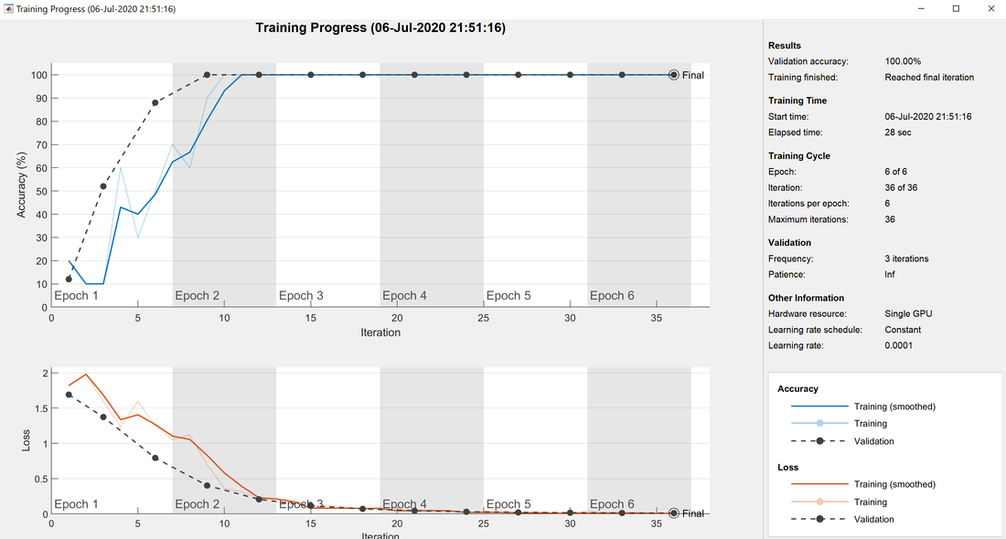
Transfer Learning Model with six epochs, 10^-4 learning rate, and 36 iterations on a single GPU.
The model shown above is re-trained with the new dataStore of images and with six epochs, 10^-4 learning rate, and 36 iterations training options and on a single GPU. The training only took 28 seconds using a GPU. This process could have taken more than two hours if you would use a CPU.
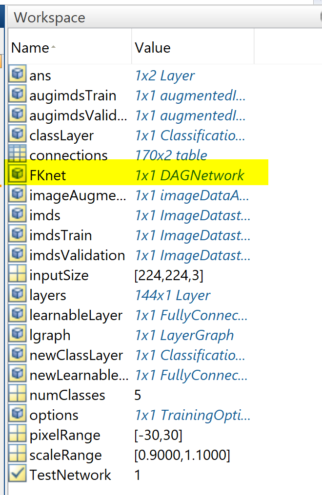
Now, the new network, FKnet can be used to classify the images over the new model. Use the code below to classify the validation images using the fine-tuned network.
%%
Next, run a Sample Test
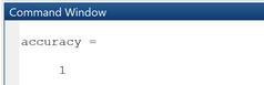
%% When you run the above code, you will get validation acuuracy of six randomely selected images as shown below.
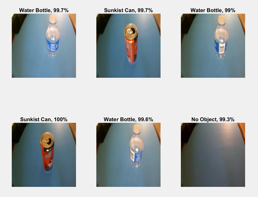
Display of six sample validation images with their predicted labels.
The confusion matrix
The confusion matrix is plotted using the "plotconfusion" function as shown below.
%% confusion plot After running the above code, you will obtain a confusion matrix chart similar to the one shown below. In our case, the model has a zero-confusion matrix that tells you about the results of the predicted label outputs comparinig to the target output.
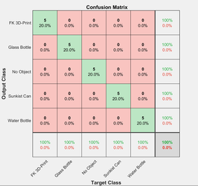
Confusion Matrix
On the confusion matrix plot, the rows correspond to the predicted class (Output Class) and the columns correspond to the true class (Target Class). The diagonal cells correspond to observations that are correctly classified. The off-diagonal cells (red) correspond to incorrectly classified observations. Both the number of observations and the percentage of the total number of observations are shown in each cell. The column on the far right of the plot shows the percentages of all the examples predicted to belong to each class that are correctly and incorrectly classified. The row at the bottom of the plot shows the percentages of all the examples belonging to each class that are correctly and incorrectly classified. The cell in the bottom right of the plot shows the overall accuracy. Note: the above results are obtained after multiple training attempts with different training options and do not expect these results on your first attempt. The video below is a complete and more advanced version of the above transfer learning tutorial. The video uses a GUI and a Matlab transfer learining APP instead of using the above codes. 3. Deep learning Video - Project # 2 | Transfer Learning »»» END of Deep Learning Part Two »»» |
|