MATLAB For Beginners
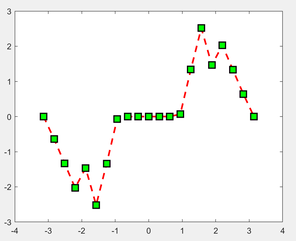
MATLAB plots plot Linear plot.
plot(X,Y) plots vector Y versus vector X. If X or Y is a matrix, then the vector is plotted versus the rows or columns of the matrix, whichever line up. If X is a scalar and Y is a vector, disconnected line objects are created and plotted as discrete points vertically at X. Various line types, plot symbols and colors may be obtained with plot(X,Y,S) where S is a character string made from one element from any or all the following 3 options: COLOR: b - blue, g - green, r - red, c - cyan, m - magenta, y - yellow, k - black, w - white SYMBOL: . point, o circle, x x-mark, + plus, * star, s square, d diamond, v triangle (down) LINE TYPE: - solid, : dotted, -. dashdot, -- dashed, (none) no line Example:
|
|
Script a:
x = 0:0.1:5; 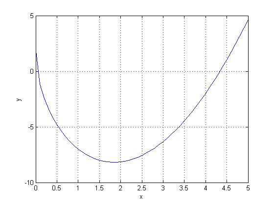
|
cript b:
x = 0:pi/100:2*pi; 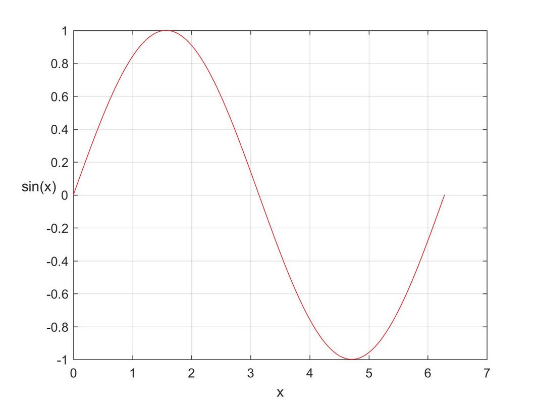
|
|
script c:
subplot(2,1,1); 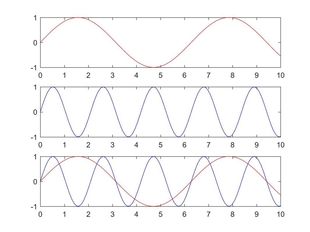
|
|
Script b:
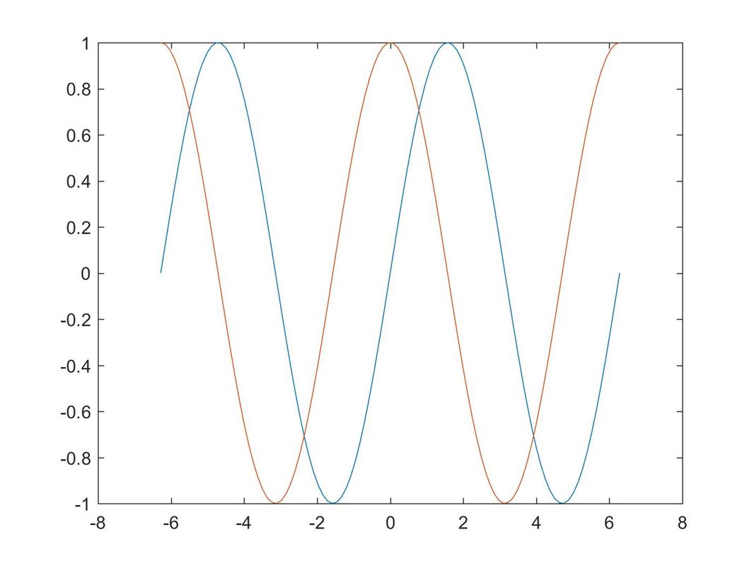
'script a' can also be modified as: x = linspace(-2*pi,2*pi); 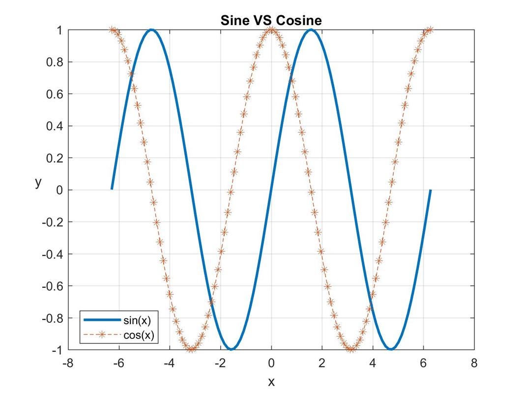
|
Script d:
'script c' can also be modified as: subplot(2,1,1); 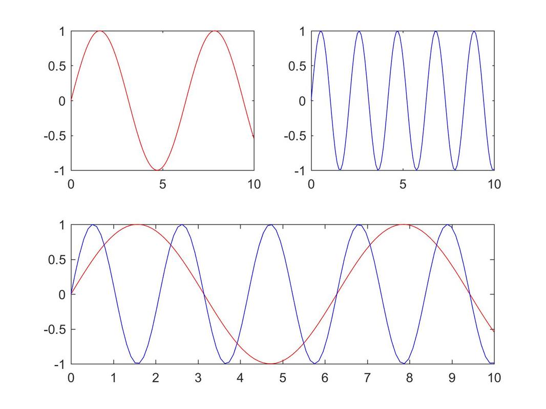
|
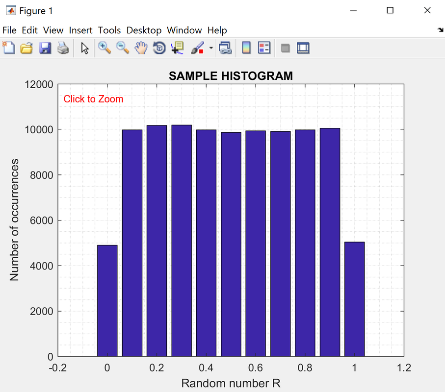
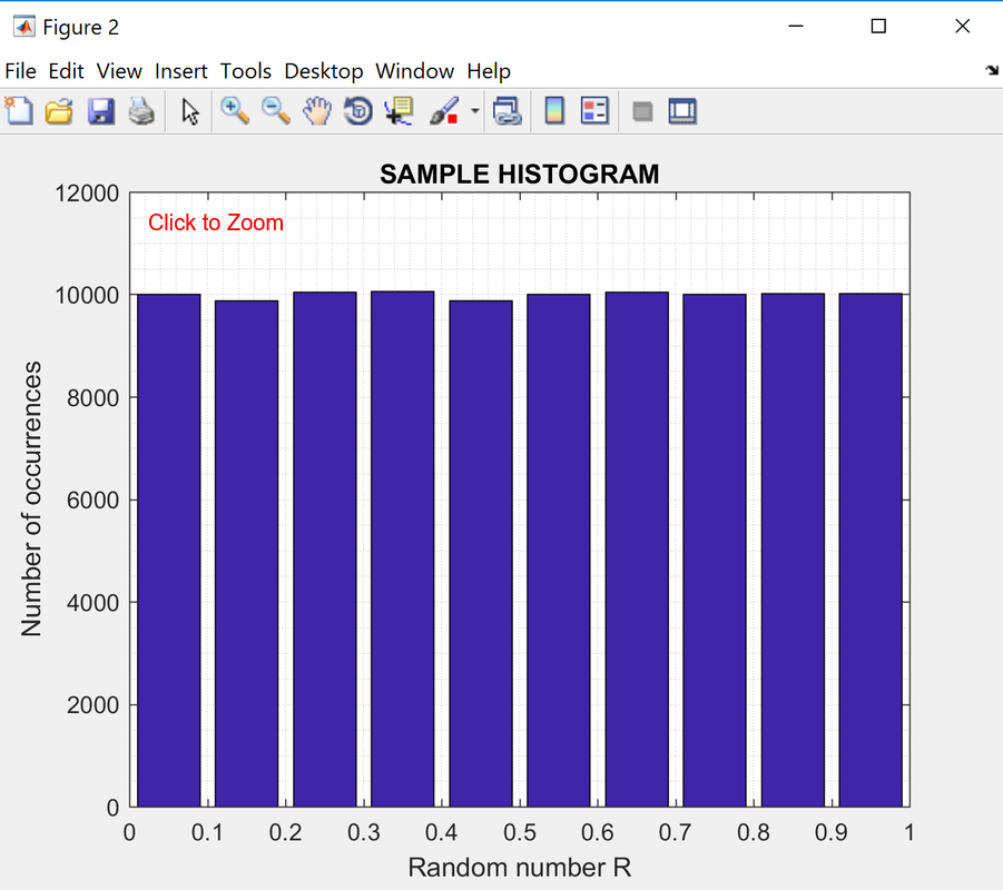
Generate N=100,000 random numbers. Then use the MATLAB “hist” function to plot the results. Depending on the limits set for the ranges of the data for the “hist” function, the histogram plots will be slightly different.
|
Matlab script:
clear; close all; |
Matlab output:
|
|
Here is the same script but for a different range.
clear; close all; |
Matlab output:
|
Back to top